How to Characterize RF Distortion
Published
How to Characterize RF Distortion, Part 2: Making Distortion Measurements
I was looking for a short article on RF measurements. I asked ChatGPT to give me an intermediate-level web article that I could read and share my thoughts on. This one caught my attention because I hadn't heard much about ACP, or Adjacent Channel Power, and revisiting the distinction between linear and nonlinear distortion is always useful. Most of my RF time has been spent trying to suppress intermodulation effects, so that part was familiar to me. I hoped to learn about some measurements I hadn't seen before and gain a new perspective on common techniques and terminology.
Eric Hsu does a great job defining distortion and goes over three types of measurements used to characterize nonlinear distortion. He defines distortion as any alteration of the original waveform. I like this way of describing it. Coming from a guitar player's perspective, this is much different. Guitar players often describe sounds by their vibe, so this definition is much clearer. It really broadens the definition. You could even call a phaser or reverb distortion.
Hearing the descriptions of linear and nonlinear distortion side by side was very clarifying. Eric goes on to say that linear distortion involves only gain and phase, while nonlinear distortion includes everything else. I would describe nonlinear distortion as something that adds, removes, or changes frequencies.
There are three types of nonlinear distortion discussed in the article, along with explanations of how to measure them.
The three types are harmonic distortion, intermodulation distortion, and Adjacent Channel Power, or ACP. I hadn't heard much about the last one. He calls these “nonlinear distortion measurements,” which was initially confusing because that also sounds like the name of the distortion itself. Maybe it is both.
Each of the three types is shown with a block diagram and a screenshot of the display from a live experiment. These are all Keysight instruments, of course, because the article is from the Keysight website.
Harmonic Distortion
For the harmonic distortion section, Figure 2 shows a harmonic measurement made with a Keysight X-Series signal analyzer. The signal analyzer is using zero span, which I am not familiar with. This is apparently a time-domain measurement that measures the fundamental tone and the subsequent harmonics. I can see the falling power level of each harmonic. It looks generally correct, but I need to look further into this type of measurement.
Third-Order Intermodulation Distortion
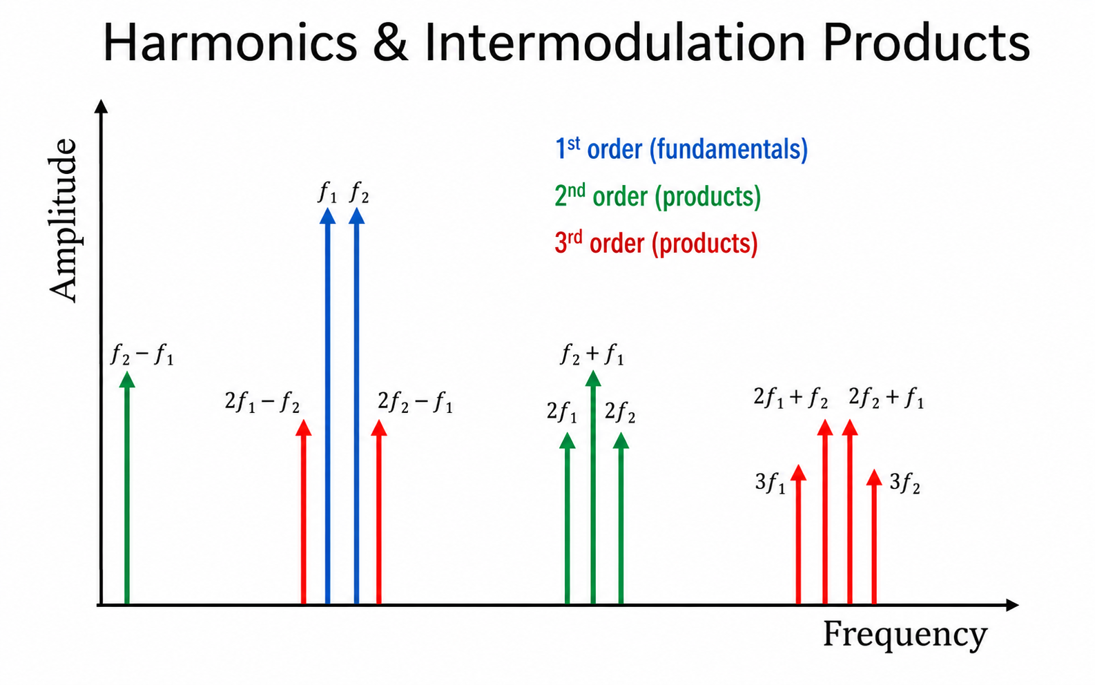
The intermodulation display is much more recognizable. We see the input waveform, which includes tones at 995 and 1005 MHz. The next tones are labeled as the upper third-order and lower third-order products. This initially did not make sense to me because I expected the second-order intermodulation products to be closest to the original tones. I will need to look further into this.
Adjacent Channel Power
The adjacent channel power section was very new to me, and the measurement did not immediately make sense. I am guessing that the green sections in the display represent the adjacent-channel measurement regions. I understand that the blue section represents the main channel, and that the measurement compares the power in the adjacent regions with the power in the main channel.
I think the most useful idea here is the reminder that we are never dealing with ideal circuits. There will always be distortion. We need to accurately characterize the unwanted products caused by the complicated waveforms we feed into our DUTs and determine how to reduce or filter them. It is also good to remind ourselves that mixing products can add together and that we should understand and anticipate where they will appear at the output.
I plan to look further into Adjacent Channel Power to understand what levels are considered acceptable and which spectrum-analyzer settings allow it to be seen clearly.